Steps 1-6

Load the R packages we will use

library(tidyverse)
library(echarts4r)
library(hrbrthemes)

Read the data in the files, drug_cos.csv, health_cos.csv in to R and assign to the variables drug_cos and health_cos, respectively

drug_cos <- read_csv("https://estanny.com/static/week6/drug_cos.csv")
health_cos <- read_csv("https://estanny.com/static/week6/health_cos.csv")

Use glimpse to get a glimpse of the data

drug_cos %>% glimpse()

Rows: 104
Columns: 9
$ ticker       <chr> "ZTS", "ZTS", "ZTS", "ZTS", "ZTS", "ZTS", "ZTS"…
$ name         <chr> "Zoetis Inc", "Zoetis Inc", "Zoetis Inc", "Zoet…
$ location     <chr> "New Jersey; U.S.A", "New Jersey; U.S.A", "New …
$ ebitdamargin <dbl> 0.149, 0.217, 0.222, 0.238, 0.182, 0.335, 0.366…
$ grossmargin  <dbl> 0.610, 0.640, 0.634, 0.641, 0.635, 0.659, 0.666…
$ netmargin    <dbl> 0.058, 0.101, 0.111, 0.122, 0.071, 0.168, 0.163…
$ ros          <dbl> 0.101, 0.171, 0.176, 0.195, 0.140, 0.286, 0.321…
$ roe          <dbl> 0.069, 0.113, 0.612, 0.465, 0.285, 0.587, 0.488…
$ year         <dbl> 2011, 2012, 2013, 2014, 2015, 2016, 2017, 2018,…

health_cos %>% glimpse()

Rows: 464
Columns: 11
$ ticker      <chr> "ZTS", "ZTS", "ZTS", "ZTS", "ZTS", "ZTS", "ZTS",…
$ name        <chr> "Zoetis Inc", "Zoetis Inc", "Zoetis Inc", "Zoeti…
$ revenue     <dbl> 4233000000, 4336000000, 4561000000, 4785000000, …
$ gp          <dbl> 2581000000, 2773000000, 2892000000, 3068000000, …
$ rnd         <dbl> 427000000, 409000000, 399000000, 396000000, 3640…
$ netincome   <dbl> 245000000, 436000000, 504000000, 583000000, 3390…
$ assets      <dbl> 5711000000, 6262000000, 6558000000, 6588000000, …
$ liabilities <dbl> 1975000000, 2221000000, 5596000000, 5251000000, …
$ marketcap   <dbl> NA, NA, 16345223371, 21572007994, 23860348635, 2…
$ year        <dbl> 2011, 2012, 2013, 2014, 2015, 2016, 2017, 2018, …
$ industry    <chr> "Drug Manufacturers - Specialty & Generic", "Dru…

Which variables are the same in both data sets

names_drug <- drug_cos %>% names()
names_health <- health_cos %>% names()
intersect(names_drug, names_health)

[1] "ticker" "name"   "year"

Select subset of variables to work with

For drug_cos select (in this order) ticker, year, grossmargin
Extract observations for 2018
Assign output to health_subset

drug_subset <- drug_cos %>% 
  select(ticker, year, grossmargin) %>% 
  filter(year == 2018)

health_subset <- health_cos %>% 
  select(ticker, year, revenue, gp, industry) %>% 
  filter(year == 2018)

Keep all the rows and columns drug_subset join with columns in health_subset

drug_subset %>% left_join(health_subset)

# A tibble: 13 × 6
   ticker  year grossmargin     revenue          gp industry          
   <chr>  <dbl>       <dbl>       <dbl>       <dbl> <chr>             
 1 ZTS     2018       0.672  5825000000  3914000000 Drug Manufacturer…
 2 PRGO    2018       0.387  4731700000  1831500000 Drug Manufacturer…
 3 PFE     2018       0.79  53647000000 42399000000 Drug Manufacturer…
 4 MYL     2018       0.35  11433900000  4001600000 Drug Manufacturer…
 5 MRK     2018       0.681 42294000000 28785000000 Drug Manufacturer…
 6 LLY     2018       0.738 24555700000 18125700000 Drug Manufacturer…
 7 JNJ     2018       0.668 81581000000 54490000000 Drug Manufacturer…
 8 GILD    2018       0.781 22127000000 17274000000 Drug Manufacturer…
 9 BMY     2018       0.71  22561000000 16014000000 Drug Manufacturer…
10 BIIB    2018       0.865 13452900000 11636600000 Drug Manufacturer…
11 AMGN    2018       0.827 23747000000 19646000000 Drug Manufacturer…
12 AGN     2018       0.861 15787400000 13596000000 Drug Manufacturer…
13 ABBV    2018       0.764 32753000000 25035000000 Drug Manufacturer…

Question: join_ticker

Start with drug_cos
Extract observations for the ticker “MRK” from drug_cos
Assign output to the variable drug_cos_subset

drug_cos_subset <- drug_cos %>% 
  filter(ticker == "MRK")

Display drug_cos_subset
drug_cos_subset
Use left_join to combine the rows and columns of drug_cos_subset with the columns of health_cos

Assign the output to combo_df

drug_cos_subset

# A tibble: 8 × 9
  ticker name  location ebitdamargin grossmargin netmargin   ros   roe
  <chr>  <chr> <chr>           <dbl>       <dbl>     <dbl> <dbl> <dbl>
1 MRK    Merc… New Jer…        0.305       0.649     0.131 0.15  0.114
2 MRK    Merc… New Jer…        0.33        0.652     0.13  0.182 0.113
3 MRK    Merc… New Jer…        0.282       0.615     0.1   0.123 0.089
4 MRK    Merc… New Jer…        0.567       0.603     0.282 0.409 0.248
5 MRK    Merc… New Jer…        0.298       0.622     0.112 0.136 0.096
6 MRK    Merc… New Jer…        0.254       0.648     0.098 0.117 0.092
7 MRK    Merc… New Jer…        0.278       0.678     0.06  0.162 0.063
8 MRK    Merc… New Jer…        0.313       0.681     0.147 0.206 0.199
# … with 1 more variable: year <dbl>

Use left_join to combine the rows and columns of drug_cos_subset with the columns of health_cos

Assign the output to combo_df

combo_df <- drug_cos_subset %>% 
  left_join(health_cos)

display: combo_df

combo_df

# A tibble: 8 × 17
  ticker name  location ebitdamargin grossmargin netmargin   ros   roe
  <chr>  <chr> <chr>           <dbl>       <dbl>     <dbl> <dbl> <dbl>
1 MRK    Merc… New Jer…        0.305       0.649     0.131 0.15  0.114
2 MRK    Merc… New Jer…        0.33        0.652     0.13  0.182 0.113
3 MRK    Merc… New Jer…        0.282       0.615     0.1   0.123 0.089
4 MRK    Merc… New Jer…        0.567       0.603     0.282 0.409 0.248
5 MRK    Merc… New Jer…        0.298       0.622     0.112 0.136 0.096
6 MRK    Merc… New Jer…        0.254       0.648     0.098 0.117 0.092
7 MRK    Merc… New Jer…        0.278       0.678     0.06  0.162 0.063
8 MRK    Merc… New Jer…        0.313       0.681     0.147 0.206 0.199
# … with 9 more variables: year <dbl>, revenue <dbl>, gp <dbl>,
#   rnd <dbl>, netincome <dbl>, assets <dbl>, liabilities <dbl>,
#   marketcap <dbl>, industry <chr>

Note: the variables ticker, name, location and industry are the same for all the observations Assign the company name to co_name

co_name <- combo_df %>% 
  distinct(name) %>% 
  pull()

Assign the company location to co_location

co_location <- combo_df %>% 
  distinct(name) %>% 
  pull()

Assign the industry to co_industry group

co_industry <- combo_df %>% 
  distinct(name) %>% 
  pull()

Put the r inline commands used in the blanks below. When you knit the document the results of the commands will be displayed in your text.

The company Merck & Co Inc is located in Merck & Co Inc and is a member of the Merck & Co Inc industry group.

Select variables (in this order): year, grossmargin, netmargin, revenue, gp, netincome

Assign the output to combo_df_subset

combo_df_subset  <- combo_df  %>% 
  select(year, grossmargin, netmargin, revenue, gp, netincome)

Create the variable grossmargin_check to compare with the variable grossmargin. They should be equal. grossmargin_check = gp / revenue Create the variable close_enough to check that the absolute value of the difference between grossmargin_check and grossmargin is less than 0.001

combo_df_subset  %>% 
  mutate(grossmargin_check = gp / revenue ,
           close_enough = abs(grossmargin_check - grossmargin) < 0.001)

# A tibble: 8 × 8
   year grossmargin netmargin     revenue          gp   netincome
  <dbl>       <dbl>     <dbl>       <dbl>       <dbl>       <dbl>
1  2011       0.649     0.131 48047000000 31176000000  6272000000
2  2012       0.652     0.13  47267000000 30821000000  6168000000
3  2013       0.615     0.1   44033000000 27079000000  4404000000
4  2014       0.603     0.282 42237000000 25469000000 11920000000
5  2015       0.622     0.112 39498000000 24564000000  4442000000
6  2016       0.648     0.098 39807000000 25777000000  3920000000
7  2017       0.678     0.06  40122000000 27210000000  2394000000
8  2018       0.681     0.147 42294000000 28785000000  6220000000
# … with 2 more variables: grossmargin_check <dbl>,
#   close_enough <lgl>

Create the variable netmargin_check to compare with the variable netmargin. They should be equal.

Create the variable close_enough to check that the absolute value of the difference between netmargin_check and netmargin is less than 0.001

combo_df_subset %>% 
  mutate(netmargin_check = netincome / revenue ,
         close_enough = abs(netmargin_check - netmargin) <0.001)

# A tibble: 8 × 8
   year grossmargin netmargin     revenue          gp   netincome
  <dbl>       <dbl>     <dbl>       <dbl>       <dbl>       <dbl>
1  2011       0.649     0.131 48047000000 31176000000  6272000000
2  2012       0.652     0.13  47267000000 30821000000  6168000000
3  2013       0.615     0.1   44033000000 27079000000  4404000000
4  2014       0.603     0.282 42237000000 25469000000 11920000000
5  2015       0.622     0.112 39498000000 24564000000  4442000000
6  2016       0.648     0.098 39807000000 25777000000  3920000000
7  2017       0.678     0.06  40122000000 27210000000  2394000000
8  2018       0.681     0.147 42294000000 28785000000  6220000000
# … with 2 more variables: netmargin_check <dbl>, close_enough <lgl>

Question: summarize_industry

Fill in the blanks

Put the command you use in the Rchunks in the Rmd file for this quiz

Use the health_cos data

For each industry calculate

mean_netmargin_percent = mean(netincome / revenue) * 100 median_netmargin_percent = median(netincome / revenue) * 100 min_netmargin_percent = min(netincome / revenue) * 100 max_netmargin_percent = max(netincome / revenue) * 100

health_cos %>% 
  group_by(industry) %>%
  summarize(mean_netmargin_percent = mean(netincome / revenue) *100,
            median_netmargin_percent = median(netincome / revenue) * 100
  )

# A tibble: 9 × 3
  industry                           mean_netmargin_… median_netmargi…
  <chr>                                         <dbl>            <dbl>
1 Biotechnology                                 -4.66             7.62
2 Diagnostics & Research                        13.1             12.3 
3 Drug Manufacturers - General                  19.4             19.5 
4 Drug Manufacturers - Specialty & …             5.88             9.01
5 Healthcare Plans                               3.28             3.37
6 Medical Care Facilities                        6.10             6.46
7 Medical Devices                               12.4             14.3 
8 Medical Distribution                           1.70             1.03
9 Medical Instruments & Supplies                12.3             14.0

mean netmargin percent for the industry “Diagnostics & Research” = 13.1% median netmargin percent percent for the industry “Diagnostics & Research” = 12.33%

***** Question: inline_ticker

Use the health_cos data

Extract observations for the ticker ZTS from health_cos and assign to the variable health_cos_subset

health_cos_subset <- health_cos %>% 
  filter(ticker == "ZTS")

Display health_cos_subset

health_cos_subset

# A tibble: 8 × 11
  ticker name      revenue     gp    rnd netincome  assets liabilities
  <chr>  <chr>       <dbl>  <dbl>  <dbl>     <dbl>   <dbl>       <dbl>
1 ZTS    Zoetis I…  4.23e9 2.58e9 4.27e8    2.45e8 5.71e 9  1975000000
2 ZTS    Zoetis I…  4.34e9 2.77e9 4.09e8    4.36e8 6.26e 9  2221000000
3 ZTS    Zoetis I…  4.56e9 2.89e9 3.99e8    5.04e8 6.56e 9  5596000000
4 ZTS    Zoetis I…  4.78e9 3.07e9 3.96e8    5.83e8 6.59e 9  5251000000
5 ZTS    Zoetis I…  4.76e9 3.03e9 3.64e8    3.39e8 7.91e 9  6822000000
6 ZTS    Zoetis I…  4.89e9 3.22e9 3.76e8    8.21e8 7.65e 9  6150000000
7 ZTS    Zoetis I…  5.31e9 3.53e9 3.82e8    8.64e8 8.59e 9  6800000000
8 ZTS    Zoetis I…  5.82e9 3.91e9 4.32e8    1.43e9 1.08e10  8592000000
# … with 3 more variables: marketcap <dbl>, year <dbl>,
#   industry <chr>

In the console, type ?distinct. Go to the help pane to see what distinct does In the console, type ?pull. Go to the help pane to see what pull does

Run the code below health_cos_subset %>% distinct(name) %>%
pull(name)

health_cos_subset  %>% 
  distinct(name) %>%  
  pull(name)

[1] "Zoetis Inc"

Assign the output to co_name

co_name <- health_cos_subset  %>% 
  distinct(name) %>% 
  pull(name)

You can take output from your code and include it in your text.

The name of the company with ticker ZTS is Zoetis Inc In following chuck
Assign the company’s industry group to the variable co_industry

co_industry <- health_cos_subset %>% 
  distinct(industry) %>% 
  pull()

This is outside the Rchunck. Put the r inline commands used in the blanks below. When you knit the document the results of the commands will be displayed in your text.

The company Zoetis Inc is a member of the Drug Manufacturers - Specialty & Generic group

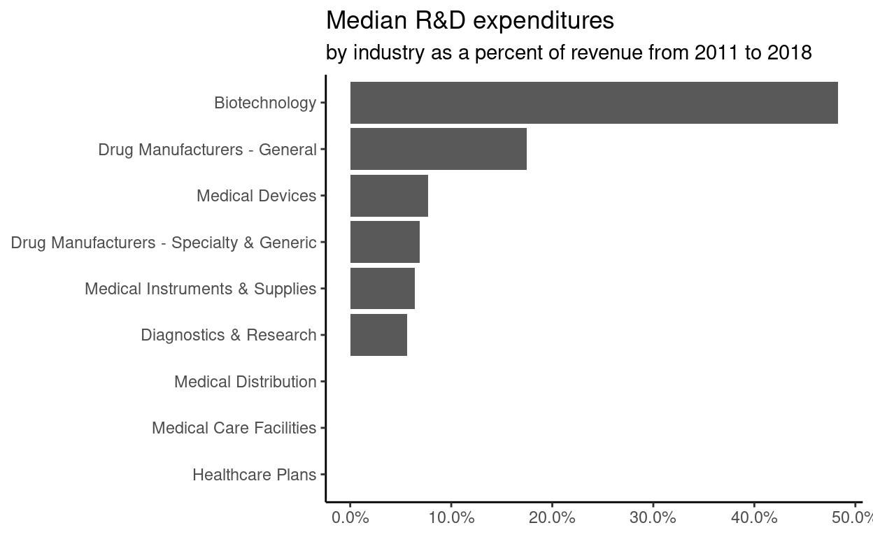
Prepare data for the plot

start with health_cos THEN gorup_by industry THEN calculate the median research and development expenditure by industry assign the output to df

df <- health_cos %>% 
  group_by(industry) %>% 
  summarize(med_rnd_rev = median(rnd/revenue))

Use glimpse to glimpse the data for the plots

df %>% glimpse()

Rows: 9
Columns: 2
$ industry    <chr> "Biotechnology", "Diagnostics & Research", "Drug…
$ med_rnd_rev <dbl> 0.48317287, 0.05620271, 0.17451442, 0.06851879, …

Create a static bar chart use ggplot to initialize the chart data is df

ggplot(data = df, 
       mapping = aes( 
         x = reorder(industry, med_rnd_rev ),
         y = med_rnd_rev
         )) +
  geom_col() + 
  scale_y_continuous(labels = scales::percent) +
  coord_flip() +
  labs(
    title = "Median R&D expenditures",
    subtitle = "by industry as a percent of revenue from 2011 to 2018",
    x= NULL, y= NULL) +
    theme_classic()

Save the last plot to preview.png and add to the yaml chunk at the top

ggsave(filename = "preview.png",
       path = here::here("_posts", "2022-03-08-joining-data"))

Create an interactive bar chart using the package echarts4r

df %>% 
  arrange(med_rnd_rev) %>% 
  e_charts(
    x = industry 
    ) %>% 
  e_bar(
    serie = med_rnd_rev, 
    name = "median"
    ) %>% 
  e_flip_coords() %>% 
  e_tooltip() %>% 
  e_title(
    text = "Median industry R&D expenditures", 
    subtext = "by industry as a percent of revenue from 2011 to 2018",
    left = "center") %>% 
  e_legend(FALSE) %>% 
  e_x_axis(
    formatter = e_axis_formatter("percent", digits = 0)
    ) %>% 
  e_y_axis(
    show = FALSE
  ) %>% 
  e_theme("infographic")

Joining data

Steps 1-6