Load the R Package we will use

library(tidyverse)
library(ggplot2)

Quiz questions Replace all the ???s. These are answers on your moodle quiz. Run all the individual code chunks to make sure the answers in this file correspond with your quiz answers After you check all your code chunks run then you can knit it. It won’t knit until the ??? are replaced The quiz assumes that you have watched the videos, downloaded (to your examples folder) and worked through the exercises in exercises_slides-1-49.Rmd Pick one of your plots to save as your preview plot. Use the ggsave command at the end of the chunk of the plot that you want to preview.

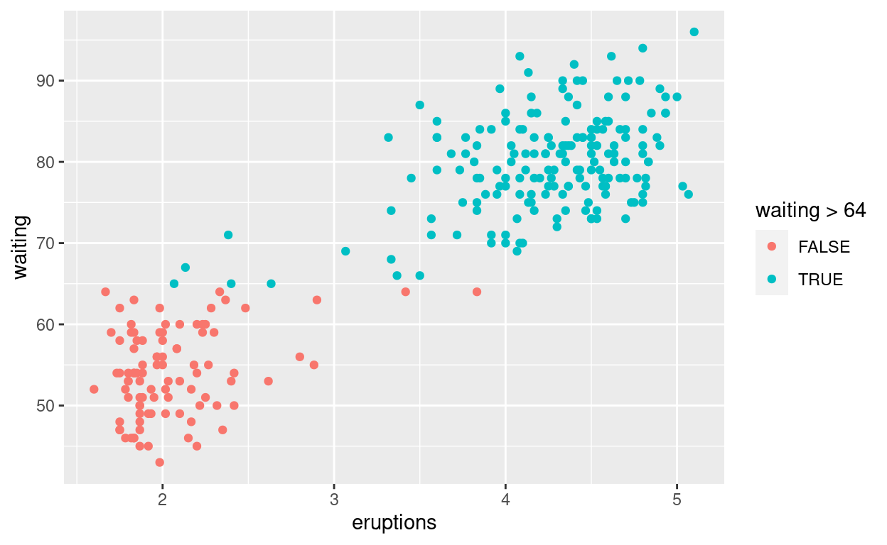
#Question: modify slide 34 34. If an aesthetic is linked to data it is put into aes()

ggplot(faithful) + 
  geom_point(aes(x = eruptions, y = waiting, colour = waiting > 64))

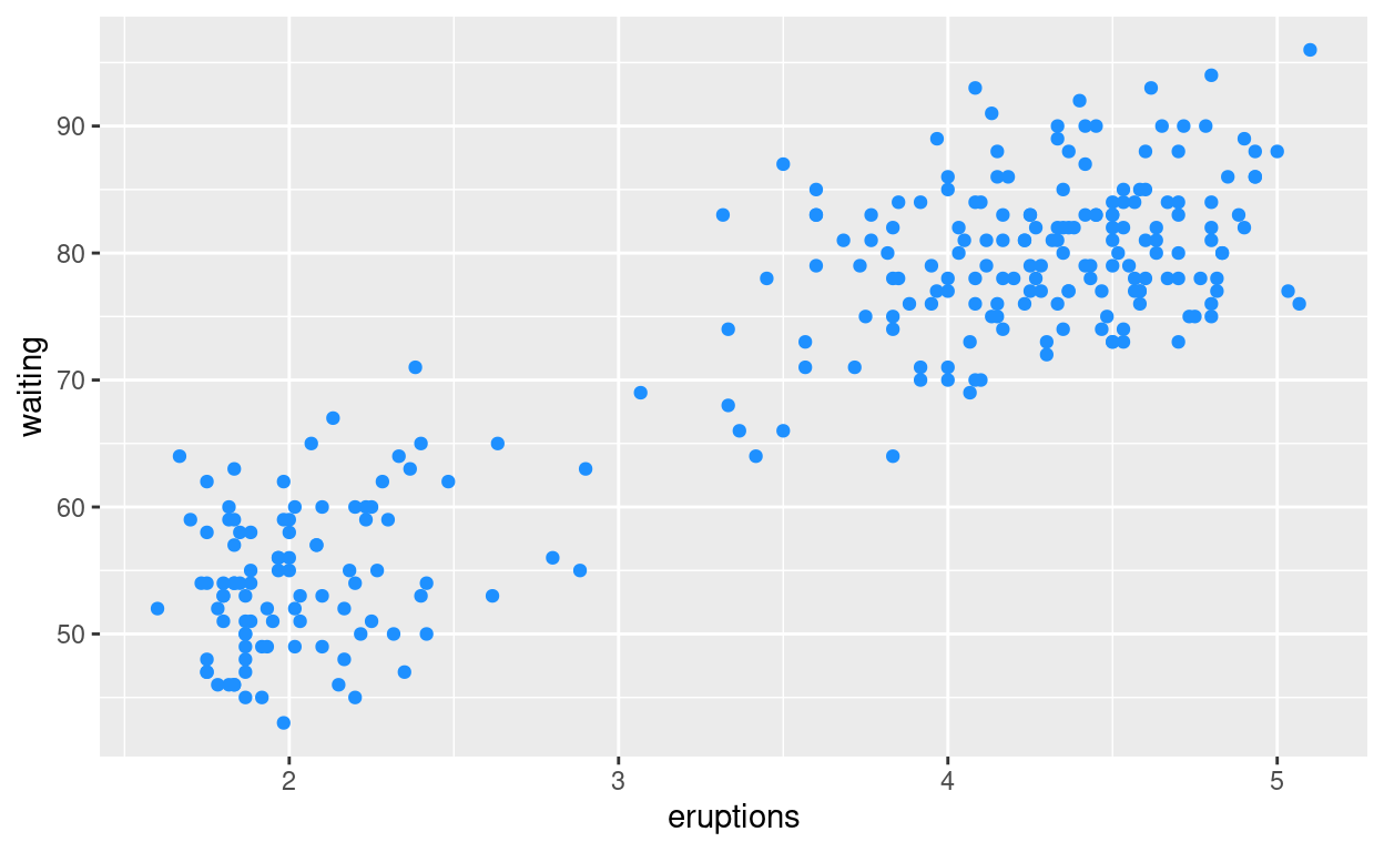
Question: modify slide 35

If you simple want to set it to a value, put it outside of aes()

ggplot(faithful) + 
  geom_point(aes(x = eruptions, y = waiting),
             colour = 'dodgerblue')

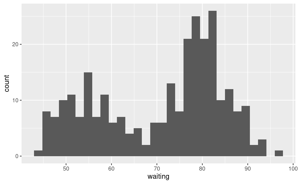
Question: modify slide 36

Some geoms only need a single mapping and will calculate the rest for you

ggplot(faithful) + 
  geom_histogram(aes(x = waiting))

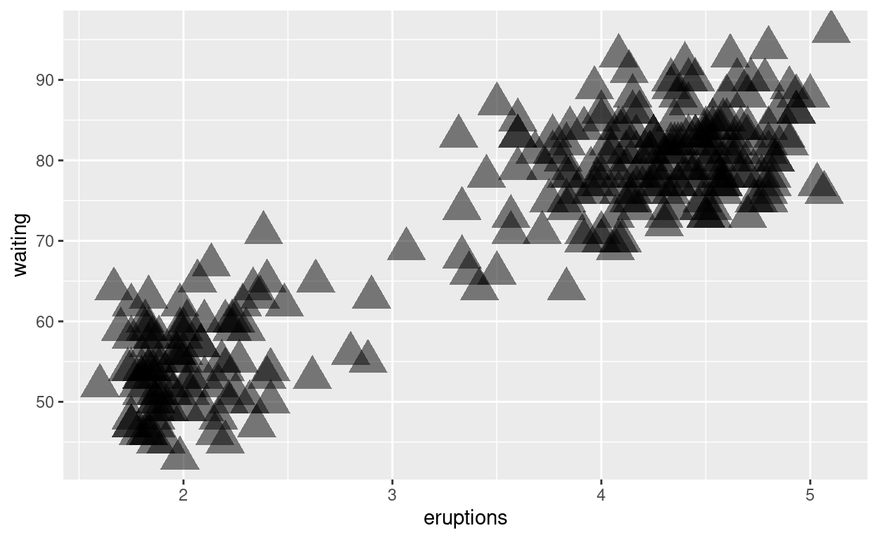
Question: modify geom-ex-1

Geom-Ex-1. Modify the code below to make the points larger squares and slightly transparent. See ?geom_point for more information on the point layer.

ggplot(faithful) + 
  geom_point(aes(x = eruptions, y = waiting),
             shape = "triangle", size = 7, alpha = 0.5)

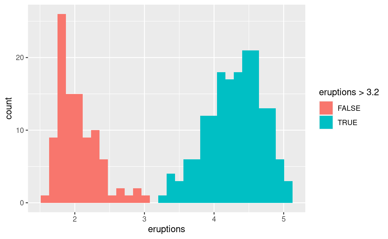
Question: modify geom-ex-2

Geom-Ex-2. Colour the two distributions in the histogram with different colours

ggplot(faithful) + 
  geom_histogram(aes(x = eruptions, fill = eruptions > 3.2))

Question: modify slide 40

Every geom has a stat. This is why new data (count) can appear when using geom_bar().

ggplot(mpg) + 
  geom_bar(aes(x = manufacturer))

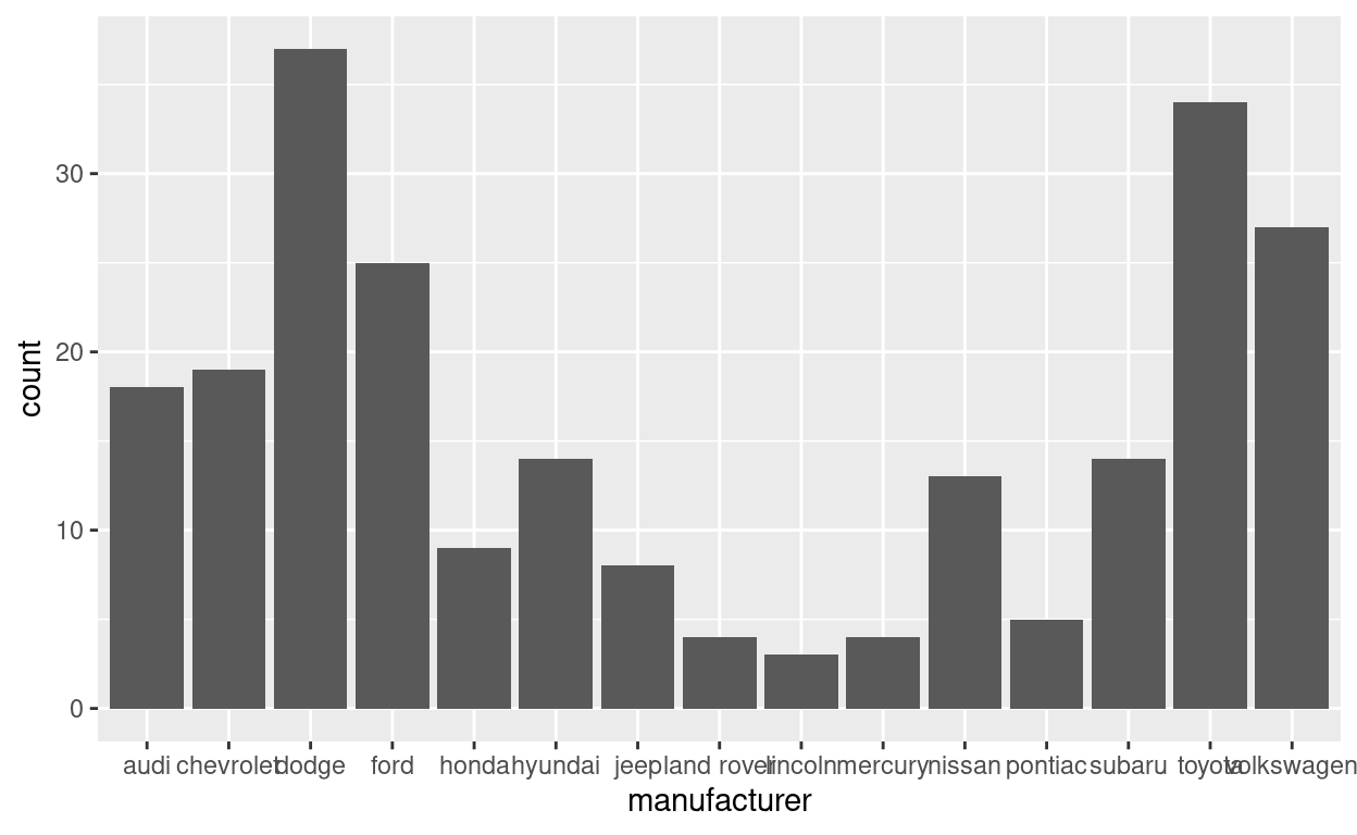
Question: modify slide 41

The stat can be overwritten. If we have precomputed count we don’t want any additional computations to perform and we use the identity stat to leave the data alone

mpg_counted <- mpg %>% 
  count(manufacturer, name = 'count')
ggplot(mpg_counted) + 
  geom_bar(aes(x = manufacturer, y = count), stat = 'identity')

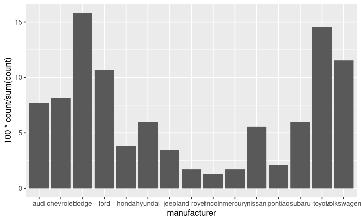
Question: modify slide 43

Values calculated by the stat is available with the after_stat() function inside aes(). You can do all sorts of computations inside that.

ggplot(mpg) + 
  geom_bar(aes(x = manufacturer, y = after_stat(100 * count / sum(count))))

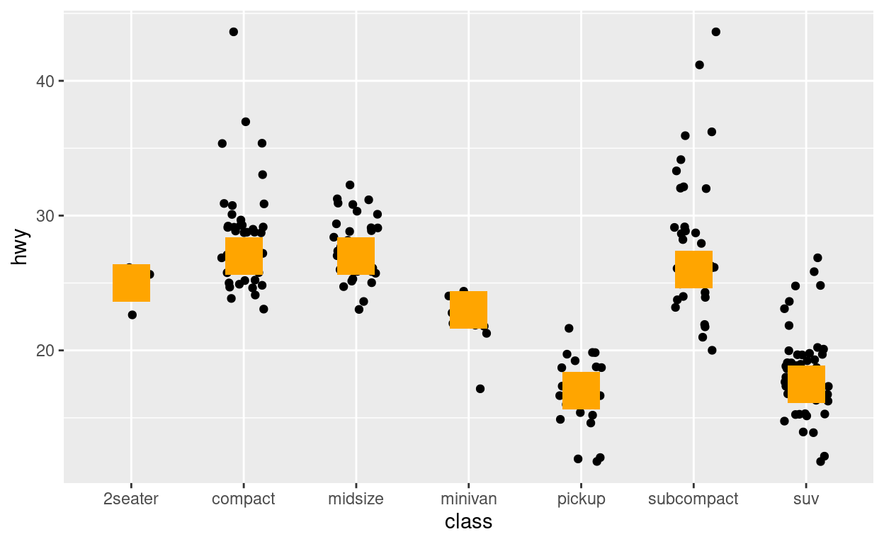
Question: modify stat-ex-2

Use stat_summary() to add a red dot at the mean hwy for each group

ggplot(mpg) + 
  geom_jitter(aes(x = class, y = hwy), width = 0.2) +
  stat_summary(aes(x = class, y = hwy), geom = "point", 
               fun = "median", color = "orange", shape = "square", size = 9)

ggsave("preview.png")

7: Exploratory analysis